Neural Image Caption Generator
The caption on the image above was generated by a neural network. More precisely, using a combination of two neural networks known as encoder-decoder architecture.
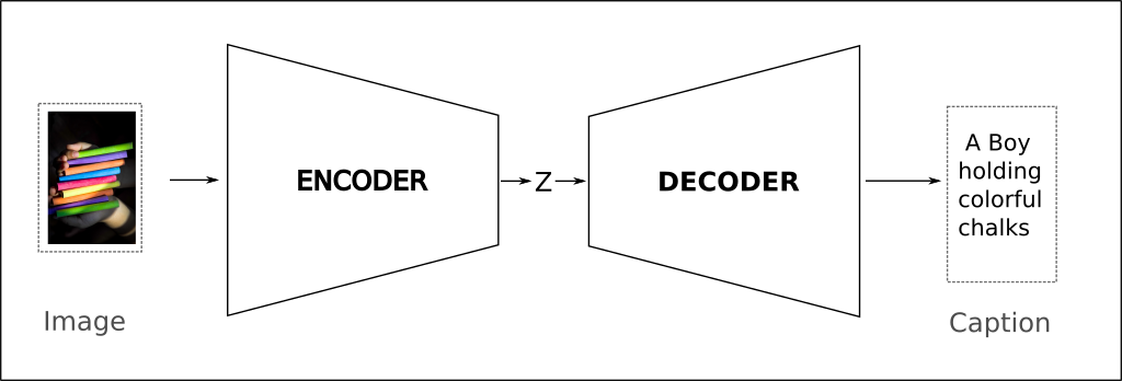
Example of the caption we want the model to generate
The natural question then is “how does the model generate captions ?”. Let’s zoom into the network architecture.
The Encoder consists of a state of the art vision model (CNN) and the Decoder is responsible for learning the language model using RNN. We pass the image through the Encoder network, where a pre-trained Convolutional Neural Network extracts the image features and converts it into the encoded feature vector (Z). The Decoder network takes Z as input and uses it along along with the hidden state of RNN to generate the caption - one word at a time.
Great, but how can it generate fully formed sentences instead of some arbitrarily placed alphabets?
The Decoder is responsible for learning two tasks - learn the structure of the language (i.e the Language Model) so that it can generate English sentences and also learn the contents of the image. The decoder must learn both the tasks together, learning one is not enough. If it only learns the language model, it will output words or fully formed sentences with no relation to the image. If it only learns to recognize the contents of the image, it will output the name of object but will not be able to describe how those objects relate to each other.
In the following section, I will describe how to build an end-to-end image captioning system using neural networks.
Show and Tell: A Neural Image Caption Generator
This paper by Vinyals et. al was perhaps one of the first to achieve state of the art results on Pascal, Flickr30K, and SBU using an end-to-end trainable neural network. As the authors highlight, the main inspiration of this paper comes from the breakthrough work in Neural Machine Translation. Machine translation, as the name suggests, is the task of translating text from one language to another.
Detour
Before 2014, the language translation was done largely using statistical machine translation (SMT) models. The core idea of statistical machine translation is to learn a probabilistic model from the training data (e.g English to Hindi Corpus):
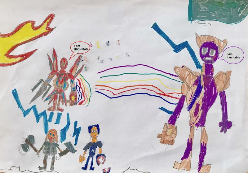
Recreation of the final battle scene from Avengers Endgame by an eight-year old
Given a sentence in English, for example the last words of Thanos in Endgame i.e (x): I am Inevitable
We want the model to translate it to Hindi sentence, (y): मैं अपरिहार्य हूं (Google Translate)
i.e on a very high level, we want
By the way, Is Avengers Endgame the best performing movie in the Marvel Cinematic Universe. I try to find out here?
SMT models required a very complex feature engineering pipeline along with several separately designed subcomponents. Each of which required lots of human effort for each language pair.
In 2014, the researchers from Google introduced an end-to-end trainable approach that used two recurrent neural networks to learn the mapping from one sequence to another. They called it sequence to sequence learning and applied it on machine translation task. The translations produced by their seq2seq model performed as good as the SMT method on the same dataset. Since then, the architecture has been applied to different domains such as speech recognition, text summarization and of course machine translation.
End of Detour
In Neural Image Caption, the authors use similar architecture but replace the RNN in encoder with CNN as Convnets tend to perform better on computer vision tasks. The main contributions of the paper are:
- End-to-end trainable system
- Use of state of the art sub-networks for vision and language models
How does it work
The diagram shows the neural network architecture that I used to implement Show and Attend paper.
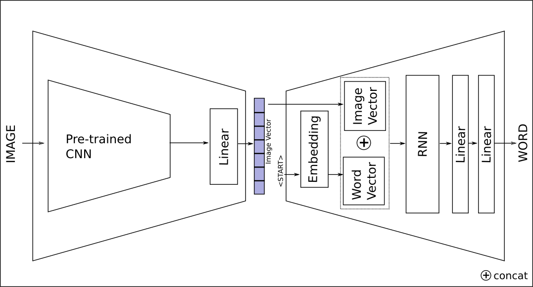
OBJECTIVE: For a given input image, the model’s objective is to maximise the probability of generating the correct sentence.
Where S is the generated sentence, I is the input image and is the model parameters. A sentence S consists to multiple words i.e. where N is total number of words in a sentence. We can then model the join probability by applying chain rule:
We train the network using image-caption pair (S,I) with the objective of maximising the sum of log probabilities as shown above. For each training example, we pass the input image through the encoder network to extract the feature vector, we then use the decoder network to generate the sentence, one word at each timestep. We concatenate the word embeddings and the image feature vector before passing them as the input to RNN, this is done to map them to the same space. And although the architecture above displays the word as output, in reality, the decoder generates the probabilities over all words in the vocab. We then pick the word using a decoding algorithm (more on this later).
At the initial timestep , we pass a special start of sentence word token (i.e =<START>) and at subsequent timesteps, we pass the image feature vector along with the word generated at the previous timestep. This means we call the decoder several times until we have the full sentence. Since the length of the sentence is unbounded, we need a mechanism to know when to stop. This is done using a special end of sentence marker i.e =<STOP>.
LOSS: We use the negative log-likelihood of the correct word as the loss function and minimize it with respect to the top layer of the encoder and all layers of the decoder network. We only use the top layer in the encoder network and not the CNN sub-network because we do not want the pre-trained CNN to forget its learned weights.
Training Details
The following plot shows the training loss and hyper-parameters used.
| Batch size | 128 |
| Optimizer | ADAM |
| Learning rate | 1e-4 |
| Training images | 177K (COCO dataset) |
| Vocab size | 36,780 words |
| Embedding size | 256 |
| Training time | ~19h on gtx1080 |
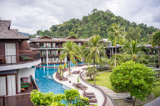
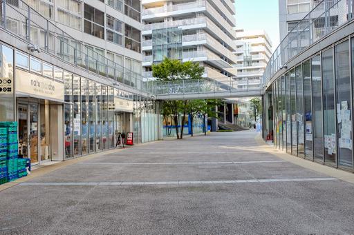
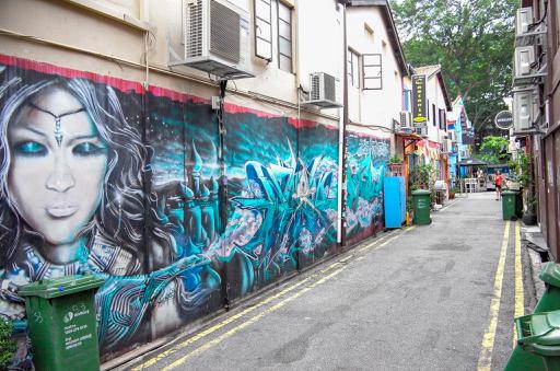
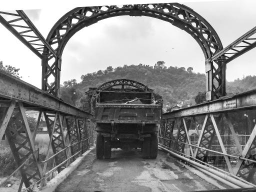
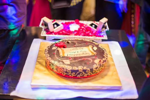
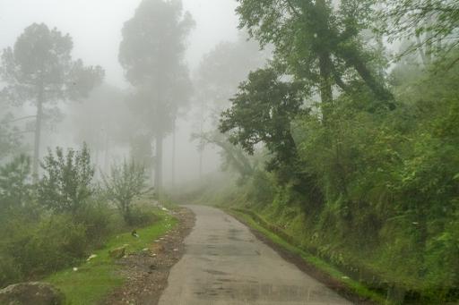
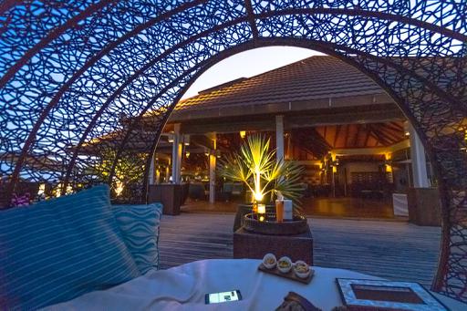
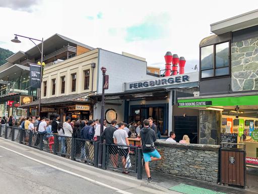
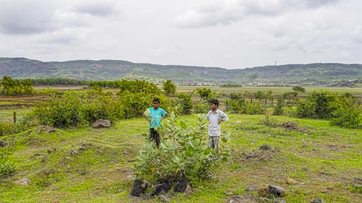
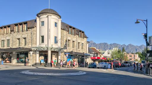
Test drive
Let’s see how well does the model perform in wild


Cherry Picked Captions, hover over the image to pause auto scroll
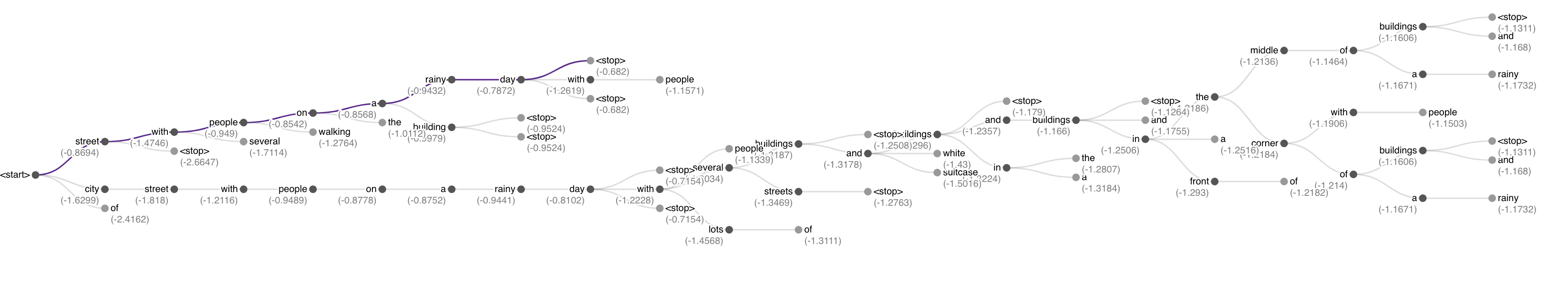
After the model is trained, there are different ways to generate the caption. Recall that at every step, the model generates the probabilities over the entire vocabulary so the easiest and the most obvious approach would be to pick the word with the highest probability. This is called greedy decoding where we greedily select the next word. And while it may be able to generate captions, there are better options available. Let’s briefly look at each of them.
Decoding Algorithms:
At every step, pick the word with the highest probability to generate the sequence. It is a simple method that generates low-quality output compared to other methods in the list.
Track multiple sequences at once. Instead of using just one word, store top k words at every step t. At the next step t+1, generate top k words for each for previous top k words. This end result is a tree of words (i.e multiple hypotheses), pick the one with the highest probability. k=1 is greedy search and suffers from the same issue of producing low-quality output, increasing k is compute intensive but generally produces higher quality output. Although at larger k, the output gets very short.
Similar to greedy decoding, but instead of picking the word with the highest probability, randomly sample the word from the probability distribution. Sampling methods such as pure sampling and top-K provide better diversity and are generally better at natural language generation.
Similar to Pure sampling, but instead of sampling just a single word, sample top-k probable words. k=1 is greedy search and k=length of vocabulary is pure sampling.
Visualization of Beam Search Decoder from here
For more details on decoding algorithms, see: Visualising Decoding Algorithms
The carousel above presented the cherry-picked image and their captions. Below we compare how each decoding algorithm performs against the baseline, which in this case is the captions generated by an 8-year old who agreed after some negotiations 🎁.


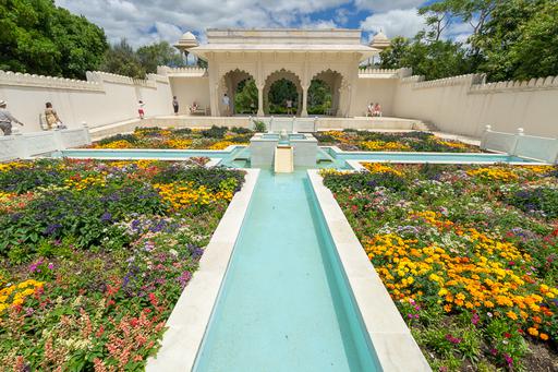


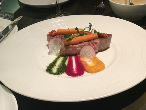

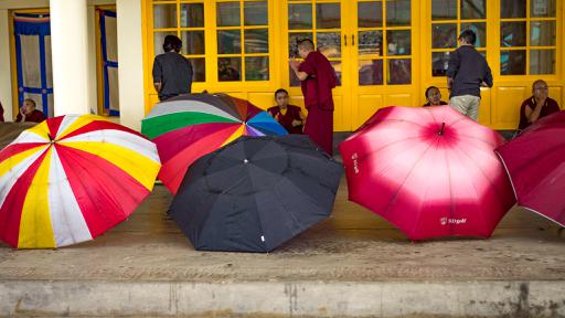
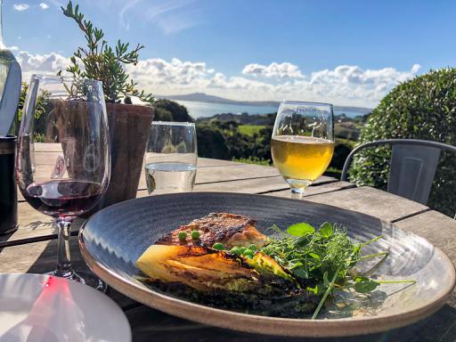


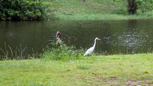
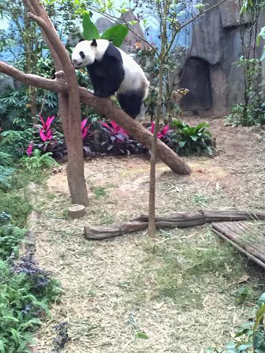
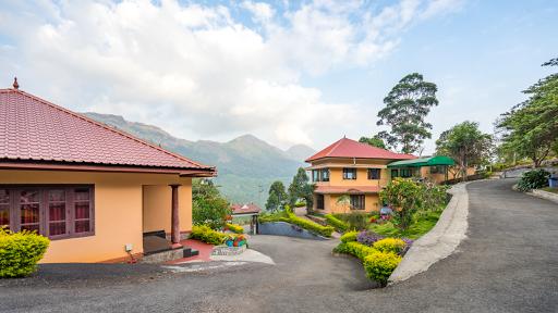

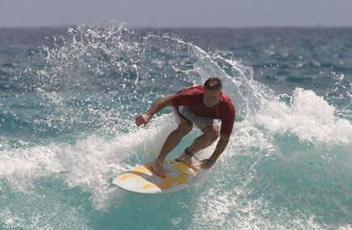
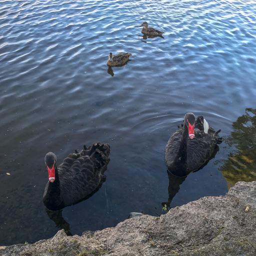
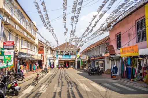


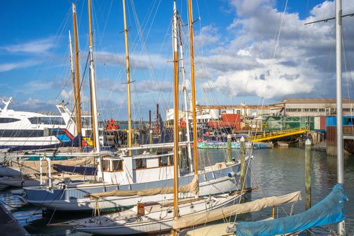
Hover over the image to view the captions
Conclusion
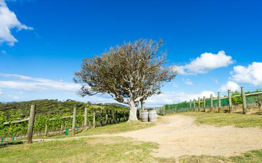
We were able to build and train a seq2seq network that was largely based on the architecture used in the show and tell paper. We tested the model on images in the wild, in this case, a sample from my collection of photos
- which is different from the dataset our model was trained on. We saw that pure sampling and top-k sampling decoders produced better captions but the overall result was not as good as we would like it to be. We can try a few things - train the model long enough, use full training set from the COCO dataset, network architecture changes and make use of attention.
Note that we did not perform any model performance comparison between the datasets using BLEU scores, this is intentional because my objective was to learn how to build an image caption system and try on a variety of images. I do plan to use BLEU scores to compare the model described in this post with the attention-based seq2seq model.
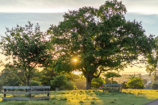
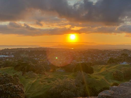
Before ending the post, here is the caption generated by the model used in this post and the new attention-based model that I just finished working on. Both the captions were generated using Greedy decoder.
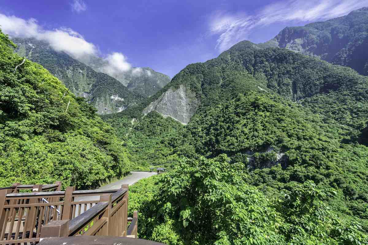
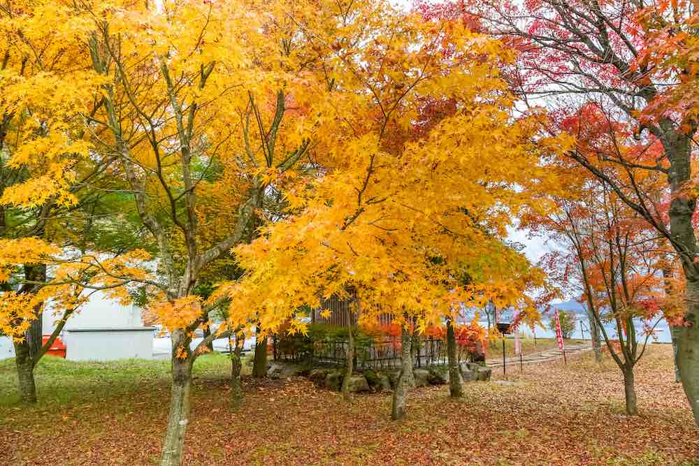
Vanilla Model: Sunset trees
Attention Model: View of mountains and a fence overlooking a mountain range
Code and model checkpoint is available on my GitHub Repo.
Check out the Part 2: Attention
REFERENCES
[1] Visualising Decoding Algorithms
[2] Show and Tell: A Neural Image Caption Generator
[3] Sequence to Sequence Learning with Neural Networks
[4] CS224N Machine Translation Lecture
[5] Tensorflow NMT Notebook