Mixture Density Networks

Supervised machine learning models learn the mapping between the input features (x) and the target values (y). The regression models predict continuous output such as house price or stock price whereas classification models predict class/category of a given input for example predicting positive or negative sentiment given a sentence or paragraph. In this notebook, we are going to focus on regression problems and work our way from predicting the target values to learning to approximate the underlying distribution.

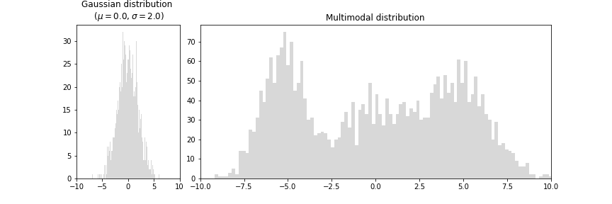
But, why learn distribution when we can directly predict the target values? Well, in most regression problems we assume the distribution of the target value to follow Gaussian distribution (left plot) but in reality, many problems have multiple modalities (right plot) that cannot be solved by directly predicting target values.

We explore this using an example presented in PRML book, where we show that a 2 layer neural network is able to approximate the target values for a given input, but fails when we invert the problem. i.e input becomes the target and vice-versa.

# Add required imports import numpy as np import matplotlib.pyplot as plt plt.style.use('default') %matplotlib inline

Toy problem

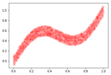
# Example presented in the PRML book def create_book_example(n=1000): # sample uniformly over the interval (0,1) X = np.random.uniform(0., 1., (n,1)).astype(np.float32) # target values y = X + 0.3 * np.sin(2 * np.pi * X) + np.random.uniform(-0.1, 0.1, size=(n,1)).astype(np.float32) # test data x_test = np.linspace(0, 1, n).reshape(-1, 1).astype(np.float32) return X, y, x_test # Plot data (x and y) X, y, x_test = create_book_example(n=4000) plt.plot(X, y, 'ro', alpha=0.04) plt.show()

Neural Network

We will use Tensorflow to build a 2-Layer neural network with fully connected layers to learn the mapping between X and y.

# Load Tensorflow import os os.environ['CUDA_VISIBLE_DEVICES'] = '0' import tensorflow as tf from copy import deepcopy # Print tensorflow version tf.__version__

‘2.0.0-dev20190208’

# Is GPU Available tf.test.is_gpu_available()

True

# Are we executing eagerly tf.executing_eagerly()

True

# Build model def get_model(h=16, lr=0.001): input = tf.keras.layers.Input(shape=(1,)) x = tf.keras.layers.Dense(h, activation='tanh')(input) x = tf.keras.layers.Dense(1, activation=None)(x) model = tf.keras.models.Model(input, x) # Use Adam optimizer model.compile(optimizer=tf.keras.optimizers.Adam(lr=lr), loss='mse', metrics=['acc']) # model.compile(loss='mean_squared_error', optimizer='sgd') return model

We could play around with model configuration to see how it impact the predictions. I am using the one described in the PRML book (page 274).

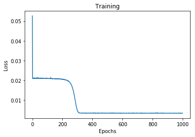
# Load and train the network model = get_model(h=50) epochs=1000 # Change verbosity (e.g verbose=1) to view the training progress history = model.fit(X, y, epochs=epochs, verbose=0) print('Final loss: {}'.format(history.history['loss'][-1])) # Plot the loss history plt.plot(range(epochs), history.history['loss']) plt.xlabel('Epochs') plt.ylabel('Loss') plt.title('Training') plt.show() Final loss: 0.0034893921427428722

With our model trained and ready for prediction, we test it on simulated data

# Predict the target values for test data and # plot along with training data y_test = model.predict(x_test) plt.plot(X, y, 'ro', alpha=0.05, label='train') plt.plot(x_test, y_test, 'bo', alpha=0.3, label='test') plt.legend(bbox_to_anchor=(1.05, 1), loc=2, borderaxespad=0.) plt.title('Plot train and test data') plt.show()

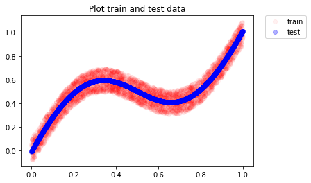
As we can see, the neural network is able to approximate well and we see the predictions following the mean of true target values

---

Inverse problem

Next, we invert the problem to investigate whether the same/similar model is able to approximate the target values.

# print data shape print(X.shape, y.shape) # Deepcopy is not required in this case # (its more of a habit for me) flipped_x = deepcopy(y) flipped_y = deepcopy(X) # load and train the model model = get_model(lr=0.09) # Train the model for large number of epochs epochs=1500 history = model.fit(flipped_x, flipped_y, epochs=epochs, verbose=0) print(history.history['loss'][-1]) plt.plot(range(epochs), history.history['loss']) plt.xlabel('Epochs') plt.ylabel('Loss') plt.title('Training') plt.show() (4000, 1) (4000, 1) 0.05178604498505592

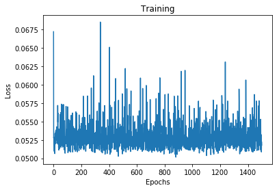
Well, the loss didn’t change much after the first few epochs, let see how well does the model perform

# epochs 500 x_test_inv = np.linspace(0., 1., 4000).reshape(-1, 1) y_test_inv = model.predict(x_test_inv) plt.plot(y, X, 'ro', alpha=0.05) plt.plot(x_test_inv, y_test_inv, 'b.', alpha=0.3) plt.show()

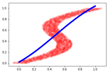
This is the best our model could do because it was confused by the non-gaussian distribution of target values. Note that there are multiple modes in the plot above.

The model could only learn to generate a linear mapping between our inverse data. This motivates the idea of learning the distribution instead of directly mapping the input and output values. The Mixture density network (MDN) does this by learning K different Gaussian parameters for every input data. We see how to implement it the next section

---

Motivation

<detour>

My motivation to learn MDN comes primarily from the world models paper by Ha and Schmidhuber. The world models paper presents a technique to train an agent, in a reinforcement learning environment, in an unsupervised manner. It makes use of three components: Variational Autoencoder to convert high dimensional space into the low dimension, MDN-RNN to compress temporal respentation and a linear model to determine what action to take to maximize cumulative reward. I intend to cover this in detail in a future post or notebook.

</detour>

MDN

In MDNs, instead of modeling the input (x) -> target (y) mapping by explicitly generating the output values, we learn the probability distribution of each target and sample the predicted output $\hat{y}$ from that distribution. The distribution itself is represented by several gaussians (i.e a mixture of gaussians). A mixture of gaussians is able to represent a complex distribution as shown in the plot titled ‘Multimodal distribution’ at the begining of this post.

For every input x, we learn the distribution parameters namely mean, variance and mixing coefficient. In terms of total output values, there are (l+2)k values where k is the number of gaussians and l is the number of input features. The breakdown of output values is shown below:

• Mixing coefficient $\pi$ : K
• Variance ($\sigma^2$) : K
• Mean($\mu$) : L * K

MDN provides a generic framework for modeling conditional probability distribution using a linear combination of mixing coefficient and respective component densities:

$p(y|x) = \sum_{k} \pi_k(x) \mathcal{N}(y|\mu_k(x),\sigma_k^2(x))$

Neural network

We use a similar neural network as used in previous examples but instead learn the mixing coefficients and component density parameters.

# In our toy example, we have single input feature l = 1 # Number of gaussians to represent the multimodal distribution k = 26 # Network input = tf.keras.Input(shape=(l,)) layer = tf.keras.layers.Dense(50, activation='tanh', name='baselayer')(input) mu = tf.keras.layers.Dense((l * k), activation=None, name='mean_layer')(layer) # variance (should be greater than 0 so we exponentiate it) var_layer = tf.keras.layers.Dense(k, activation=None, name='dense_var_layer')(layer) var = tf.keras.layers.Lambda(lambda x: tf.math.exp(x), output_shape=(k,), name='variance_layer')(var_layer) # mixing coefficient should sum to 1.0 pi = tf.keras.layers.Dense(k, activation='softmax', name='pi_layer')(layer)

Display model summary for inspection.

model = tf.keras.models.Model(input, [pi, mu, var]) optimizer = tf.keras.optimizers.Adam() model.summary() Model: "model_11" __________________________________________________________________________________________________ Layer (type) Output Shape Param # Connected to ================================================================================================== input_12 (InputLayer) [(None, 1)] 0 __________________________________________________________________________________________________ baselayer (Dense) (None, 50) 100 input_12[0][0] __________________________________________________________________________________________________ dense_var_layer (Dense) (None, 26) 1326 baselayer[0][0] __________________________________________________________________________________________________ pi_layer (Dense) (None, 26) 1326 baselayer[0][0] __________________________________________________________________________________________________ mean_layer (Dense) (None, 26) 1326 baselayer[0][0] __________________________________________________________________________________________________ variance_layer (Lambda) (None, 26) 0 dense_var_layer[0][0] ================================================================================================== Total params: 4,078 Trainable params: 4,078 Non-trainable params: 0 __________________________________________________________________________________________________

Loss

The loss function with respect to component weights w is given by $L(w) = \frac{-1} {N} \sum_{n=1}^{N} log \{ \sum_{k} \pi_k(x_n,w)) \mathcal{N}(y_n|\mu_k(x_n, w),\sigma_k^2(x_n, w))\}$

The component density is given by $f(x) = \frac {e^ \frac {-({x-\mu})^2} {2 \sigma^2} } {\sqrt{2\pi\sigma^2}}$

Always handy to keep the latex in front during implementation.

Although the following two functions now look reasonably intuitive, it took me several hours to get it right. Without the eager mode, it would have taken me a lot longer to debug and identify the issue.

# Take a note how easy it is to write the loss function in # new tensorflow eager mode (debugging the function becomes intuitive too) def calc_pdf(y, mu, var): """Calculate component density""" value = tf.subtract(y, mu)**2 value = (1/tf.math.sqrt(2 * np.pi * var)) * tf.math.exp((-1/(2*var)) * value) return value def mdn_loss(y_true, pi, mu, var): """MDN Loss Function The eager mode in tensorflow 2.0 makes is extremely easy to write functions like these. It feels a lot more pythonic to me. """ out = calc_pdf(y_true, mu, var) # multiply with each pi and sum it out = tf.multiply(out, pi) out = tf.reduce_sum(out, 1, keepdims=True) out = -tf.math.log(out + 1e-10) return tf.reduce_mean(out)

Lets verify whether our implementation is correct by comparing the values with numpy version

# calc_pdf(3.0, 0.0, 1.0).numpy() calc_pdf(np.array([3.0]), np.array([0.0, 0.1, 0.2]), np.array([1.0, 2.2, 3.3])).numpy()

array([0.00443185, 0.03977444, 0.06695205])

# Numpy version def pdf_np(y, mu, var): n = np.exp((-(y-mu)**2)/(2*var)) d = np.sqrt(2 * np.pi * var) return n/d print('Numpy version: ') pdf_np(3.0, np.array([0.0, 0.1, 0.2]), np.array([1.0, 2.2, 3.3]))

Numpy version: array([0.00443185, 0.03977444, 0.06695205])

We also verify that MDN loss function works as expected

loss_value = mdn_loss( np.array([3.0, 1.1]).reshape(2,-1).astype('float64'), np.array([[1.0, 0.0, 0.0], [1.0, 0.0, 0.0]]).reshape(2,-1).astype('float64'), np.array([[0.0, 0.1, 0.2], [0.0, 0.1, 0.2]]).reshape(2,-1).astype('float64'), np.array([[1.0, 2.2, 3.3], [1.0, 2.2, 3.3]]).reshape(2,-1).astype('float64') ).numpy() assert np.isclose(loss_value, 3.4714, atol=1e-5), 'MDN loss incorrect'

Train

While the current dataset is small enough to be used directly, here we use the dataset API because it is trivial to load data from numpy using dataset API.

# Use Dataset API to load numpy data (load, shuffle, set batch size) N = flipped_x.shape[0] dataset = tf.data.Dataset \ .from_tensor_slices((flipped_x, flipped_y)) \ .shuffle(N).batch(N)

We will use the tf.function decorator to convert python code into tensorflow graph code (the goodness of keras API and eager execution makes tensorflow 2.0 a lot more fun)

@tf.function def train_step(model, optimizer, train_x, train_y): # GradientTape: Trace operations to compute gradients with tf.GradientTape() as tape: pi_, mu_, var_ = model(train_x, training=True) # calculate loss loss = mdn_loss(train_y, pi_, mu_, var_) # compute and apply gradients gradients = tape.gradient(loss, model.trainable_variables) optimizer.apply_gradients(zip(gradients, model.trainable_variables)) return loss

Define the model and main training loop.

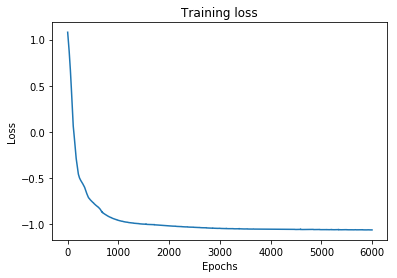
losses = [] EPOCHS = 6000 print_every = int(0.1 * EPOCHS) # Define model and optimizer model = tf.keras.models.Model(input, [pi, mu, var]) optimizer = tf.keras.optimizers.Adam() # Start training print('Print every {} epochs'.format(print_every)) for i in range(EPOCHS): for train_x, train_y in dataset: loss = train_step(model, optimizer, train_x, train_y) losses.append(loss) if i % print_every == 0: print('Epoch {}/{}: loss {}'.format(i, EPOCHS, losses[-1])) print every 600 epochs Epoch 0/6000: loss 1.0795997381210327 Epoch 600/6000: loss -0.8137094378471375 Epoch 1200/6000: loss -0.9803442358970642 Epoch 1800/6000: loss -1.0087451934814453 Epoch 2400/6000: loss -1.0302231311798096 Epoch 3000/6000: loss -1.0441244840621948 Epoch 3600/6000: loss -1.051422357559204 Epoch 4200/6000: loss -1.0547912120819092 Epoch 4800/6000: loss -1.0570876598358154 Epoch 5400/6000: loss -1.0589677095413208 # Let's plot the training loss plt.plot(range(len(losses)), losses) plt.xlabel('Epochs') plt.ylabel('Loss') plt.title('Training loss') plt.show()

Next, we predict the mixing coefficients and the component density parameters ($\mu, \sigma^2$) for test data and visualize the approximate conditional mode.

def approx_conditional_mode(pi, var, mu): """Approx conditional mode Because the conditional mode for MDN does not have simple analytical solution, an alternative is to take mean of most probable component at each value of x (PRML, page 277) """ n, k = pi.shape out = np.zeros((n, l)) # Get the index of max pi value for each row max_component = tf.argmax(pi, axis=1) for i in range(n): # The mean value for this index will be used mc = max_component[i].numpy() for j in range(l): out[i, j] = mu[i, mc*(l+j)] return out # Get predictions pi_vals, mu_vals, var_vals = model.predict(x_test) pi_vals.shape, mu_vals.shape, var_vals.shape # Get mean of max(mixing coefficient) of each row preds = approx_conditional_mode(pi_vals, var_vals, mu_vals) # Plot along with training data fig = plt.figure(figsize=(8, 8)) plt.plot(flipped_x, flipped_y, 'ro') plt.plot(x_test, preds, 'g.') # plt.plot(flipped_x, preds2, 'b.') plt.show()

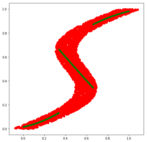
The mean of most probable density (approx conditional mode) looks promising as it does seem to capture different modalities present in the target values.

# Display all mean values # fig = plt.figure(figsize=(8, 8)) # plt.plot(flipped_x, flipped_y, 'ro') # plt.plot(x_test, mu_vals, 'g.', alpha=0.1) # plt.show()

Now that we have learned the distribution for each input value, we can sample a number of points (e.g 10) from the distribution and generate a dense set of predictions instead of picking just one.

def sample_predictions(pi_vals, mu_vals, var_vals, samples=10): n, k = pi_vals.shape # print('shape: ', n, k, l) # place holder to store the y value for each sample of each row out = np.zeros((n, samples, l)) for i in range(n): for j in range(samples): # for each sample, use pi/probs to sample the index # that will be used to pick up the mu and var values idx = np.random.choice(range(k), p=pi_vals[i]) for li in range(l): # Draw random sample from gaussian distribution out[i,j,li] = np.random.normal(mu_vals[i, idx*(li+l)], np.sqrt(var_vals[i, idx])) return out sampled_predictions = sample_predictions(pi_vals, mu_vals, var_vals, 10)

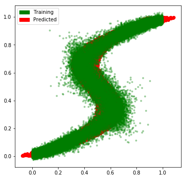
And, we see that our network has learned the approximate the multimodal distribution rather well.

# Plot the predictions along with the flipped data import matplotlib.patches as mpatches fig = plt.figure(figsize=(6, 6)) plt.plot(flipped_x, flipped_y, 'ro', label='train') for i in range(sampled_predictions.shape[1]): plt.plot(x_test, sampled_predictions[:, i], 'g.', alpha=0.3, label='predicted') patches = [ mpatches.Patch(color='green', label='Training'), mpatches.Patch(color='red', label='Predicted') ] plt.legend(handles=patches) plt.show()

Conclusion

In this post, we saw how multi modal regression problems can be solved using mixture density networks. We also saw that imperative programming environment in tensorflow 2.0 provides a pythonic way of writing code and autograph decorator allows us to convert the python code into the performant tensorflow graph.

Tensorflow 2.0, exciting times ahead.

---