CONTINUOUS CONTROL WITH DEEP REINFORCEMENT LEARNING
In this post, we are going to solve Reacher, a unity ml-agent environment, using deep deterministic policy gradient (DDPG) method introduced by Lillicrap et al.
Reacher
In this environment, a double-jointed arm can move to target locations. A reward of +0.1 is provided for each step that the agent's hand is in the goal location. Thus, the goal of our agent is to maintain its position at the target location for as many time steps as possible.
The observation space consists of 33 variables corresponding to position, rotation, velocity, and angular velocities of the arm. Each action is a vector with four numbers, corresponding to torque applicable to two joints. Every entry in the action vector should be a number between -1 and 1. This means that environment requires the agent to learn from high dimensional state space and perform actions in continuous action space.
Previously we looked at value based methods such as DQN and simple policy based methods such as hill climbing algorithm to solve environments with continuous state space but discrete action space. It turns out that neither algorithm is well suited to solve Reacher; DQN will require finding an action that maximizes the action-value which in turn requires iterative optimization process at every step; hill climbing methods could take forever as they rely on randomly perturbing the policy weights.
REINFORCE, policy based method, can learn the policy to map state into actions but they are sample inefficient, noisy because we are sampling a trajectory (or a few trajectories) which may not truly represent the policy and could prematurely converge to local optima.
Deep deterministic policy gradients
The Deep deterministic policy gradients paper introduced a model free, off-policy actor-critic algorithm that uses deep neural networks to learn policies in high-dimensional, continuous action spaces.
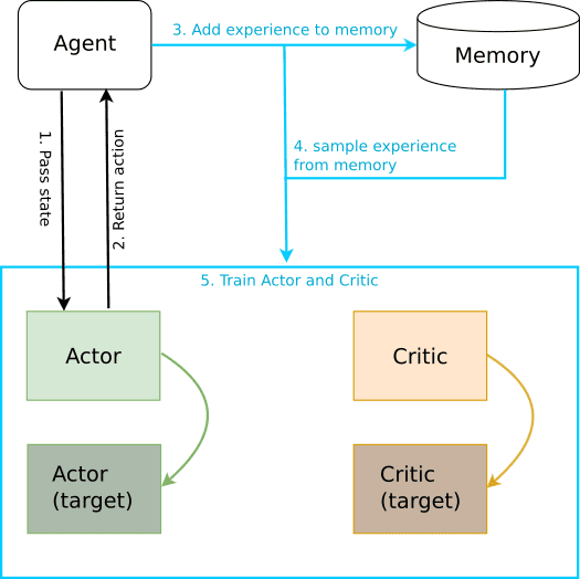
In the diagram below, I have outlined the training process. The agent is trained for the fixed number of episodes and with in each episode, fixed number of timesteps:
For fixed number of timesteps in an episode, do
Choose an action for the given state (step 1 and step 2)
Take action and receive next state, reward, done (whether episode finished?)
Store the current state, action, next state, reward and done as experience tuple in memory buffer (step 3)
Sample random batch of experience (i.e length of memory > batch size, step 4)
Train Actor and Critic networks using sampled minibatch
Training Actor and Critic Network
The actor network takes state as input and returns the action whereas the critic network takes state and action as input and returns the value. The critic in this case is a DQN with local and fixed target networks and replay buffer (memory). Both, actor and critic use two neural networks: local and fixed. The local networks are trained by sampling experiences from replay buffer and minimising the loss function.
This is how I understood the loss functions for actor and critic
The critic loss is given by
L=N1∑i(yi−Q(si,ai∣θQ))2The average of squared differences between the target action-value and the expected action-value where the expected action-value is given by the local critic network that takes state and action as input
and target action-value is calculated as
yi=ri+γQ′(si+1,μ′(si+1∣θμ′)∣θQ′)calculate the target estimate by adding the reward and discounted action-value where the target critic network takes state and action as input and returns the action-value.The target actor network maps the state to action.
The actor is updated using sampled policy gradient.
∇θμJ≈N1∑i∇aQ(s,a∣θQ)∣s=si,a=μ(si)∇θμμ(s∣θμ)The average of action-values given by the local critic network that takesstate and action as input where the action is estimated by the local actor network that takes state as input
The target networks in DQN paper were update by directly copying all the weights from local network, but in this paper, they use soft updates to constraint the target values to update slowly as it greatly improves the learning stability.
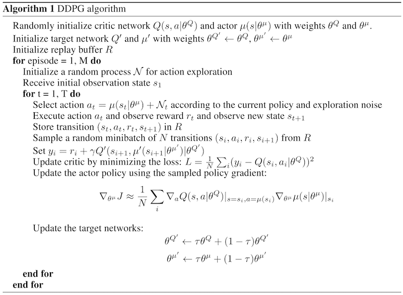
The following image from the paper shows the full algorithm
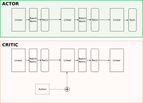
Network architecture
We use a simple network architecture because we are using raw state values as input instead of pixels. Hence, it is entirely possible to train this network on CPU. If we were to learn from pixels then we would have choosen convolutional layers along with linear.
Training
The single agent version was trained on 8-core CPU machine and the final version of the model took 36 minutes to solve the environment. However, before coming up with the final version, there was a long period of trial and error, to find out the right set of hyperparameters and network capacity. During this period, I found the following items helpful in organising my experiments.
1. Keep track of experiments
Create a new folder every time an experiment is run. Record hyperparameters, network architecture and comments along with the verbose log file. Save desired metrics as csv for analysis later (example).
2. Get real-time feedback
Publish real-time metrics, messages to visdom server for live visualisation. Sample screenshot of visdom during the training run.
3. Model checkpoint
Save model weights on every improvement over the current best score. This way I could pause the training and continue later by loading the saved model, it also gave me the flexiblity of using the saved model as starting point in some trials rather than training everything from the scratch everytime.
Final Model
This section lists the hyperparameters used in the final model. The model was able to solve the environment in 203 episodes where each episode was trained for 1000 timesteps.
Hyperparameters
Parameter
Value
Description
BATCH_SIZE
256
Minibatch size
GAMMA
0.9
Discount factor
TAU
1e-3
Soft update of target parameters
LR_ACTOR
1e-3
Actor learning rate
LR_CRITIC
1e-3
Critic learning rate
WEIGHT_DECAY
0
L2 weight decay
SCALE_REWARD
1.0
Reward scaling (1.0 means no scaling)
SIGMA
0.01
OU Noise standard deviation
FC1
128
Input channels for 1st hidden layer
FC2
128
Input channels for 2nd hidden layer
Below, we see the average score received by the agent during its training process.
Multi Agent Environment
The multi agent reacher environment includes twenty agents and presents a different challenge. The environment is considered solved when the average score of all twenty agents is +30 or above over 100 episodes. In order to solve this environment, we make use of twenty actor-critic networks but shared replay buffer because the experience tuple experienced by each agent can be useful to others.
The network architecture and hyperparameters largely remain the same but it took a lot more trials to get the agent to solve the environment. This was mainly because the agent learned very slowly e.g. improvement from 22.36 to 22.37 took 20 minutes and this lead me to "stop the training, tune hyperparameters and try again" loop. This is where the model checkpointing came in handy because I could start training from where the last training process was stopped (i.e killed) and try out different hyperparams (e.g learning rate, weight decay).
In the end, it took 28 hours of training (not including failed trials) to solve this environment. The training metrics and logs are available on my github repo. The following video shows the trained agents in action.
Future work
Some people were able to solve the environment in relatively fewer number of training episodes. I think a combination of following could help speed up the training process:
reduce network size either by remove one hidden layer or decreasing the number of units as this would result in a lot less parameters
increase the learning rate and introduce weight decay (currently set to 0) to speed up the learning
experiment with scaled rewards (see below)
This paper found that DDPG is less stable than batch algorithms such as REINFORCE and the performance of policy could degrade significantly during the training phase. In my tests, I found that average score plateaued if I continued the training process even after solving the environment. The paper also suggests that scaling the rewards could improve the training stability.
While working on DDPG solution, there were a lot of moving parts such as network architecture, hyperparameters and it took a long time, along with incorporating suggestions from the forum, to discover the combination that could solve the environment. Proximal policy optimization (PPO) has shown to achieve state-of-the-art results with very little hyperparamter tuning and greater sample efficiency while keeping the policy deviation under check (by forcing the ratio of old and new policy with in a small interval).
The code along with model checkpoints is available on my github repository.